When working with Amazon Neptune, performance tuning can often feel like navigating a dark cave without a flashlight. Queries might slow down unexpectedly, or your Gremlin traversal that worked on a small dataset suddenly takes forever on a production graph. Fortunately, Neptune gives us a tool to turn on the light: the EXPLAIN command.
In this blog, we’ll explore how to use EXPLAIN or PROFILE plans across Neptune’s three query languages (Gremlin, SPARQL, and openCypher) to diagnose performance issues, understand query execution, and optimize your graph workloads.
Why Neptune EXPLAIN and PROFILE Matter
Unlike relational databases, graph queries often involve traversals over many edges, dynamic filtering, and pattern matching. This makes performance harder to predict, and traditional indexing strategies don’t always apply. That’s where the query planner comes in: it tells you how Neptune is interpreting your query and where it might be wasting time.
How to Generate Neptune EXPLAIN Plans
Let’s look at how to generate Neptune EXPLAIN plans in each supported language.
Gremlin
In Gremlin, you generate a PROFILE plan using the profile HTTP endpoint in the Neptune Workbench or any Gremlin-compatible prompt supporting Neptune extensions. Using PROFILE rather than EXPLAIN runs the query in real-time giving you more valuable statistics:
POST https://<your-neptune-endpoint>:<port>/gremlin/profile \
     -d '{
           "gremlin":"g.V().hasLabel(\"city\")
                               .has(\"name\", \"London\")
                               .emit()
                               .repeat(in().simplePath())
                               .times(2)
                               .limit(100)"
        }'
If you are using a Jupyter Notebook to run this code, you can use the magic cell command instead:
%%gremlin profile
This runs the query and returns a full profile report including:
- Execution steps
- Durations and counts
- Optimized and physical query plans
- Traversal and repeat metrics
Sample Output (Truncated for Clarity):
>>> Neptune Explain Plan – Expand
Query String
==================

g.V().hasLabel("city").has("name", "London").emit().repeat(in().simplePath()).times(2).limit(100)

Original Traversal
==================
[GraphStep(vertex,[]), HasStep([...]), RepeatStep(...), RangeGlobalStep(0,100)]

Optimized Traversal
===================
Neptune steps:
[
  NeptuneGraphQueryStep(Vertex) {
    JoinGroupNode {
      PatternNode[(?1, <name>, "London", ?) . project ?1 .], {...}
      PatternNode[(?1, <~label>, ?2=<city>, <~>) . project ask .], {...}
      RepeatNode {
        Repeat {
          PatternNode[(?3, ?5, ?1, ?6) . project ?1,?3 . SimplePathFilter(?1, ?3)) .], {...}
        }
        Emit { Filter(true) }
        LoopsCondition { LoopsFilter([?1, ?3], eq(2)) }
      }
    }, finishers=[limit(100)]
  },
  NeptuneTraverserConverterStep
]

Physical Pipeline
=================
NeptuneGraphQueryStep
  |-- JoinGroupOp
      |-- DynamicJoinOp(...)
      |-- RepeatOp
          |-- BindingSetQueue (Iteration 1)...
          |-- BindingSetQueue (Iteration 2)...
  |-- LimitOp(100)

Runtime (ms)
============
Query Execution:  392.686
Serialization:   2636.380

Traversal Metrics
=================
Step                            Count  Traversers   Time (ms)    % Dur
--------------------------------------------------------------
NeptuneGraphQueryStep(Vertex)    100         100      314.162    82.78
NeptuneTraverserConverterStep    100         100       65.333    17.22
TOTAL                               -           -      379.495       -

Repeat Metrics
==============
Iteration  Visited   Output    Until     Emit     Next
------------------------------------------------------
        0        1        1        0        1        1
        1       61       61        0       61       61
        2       38       38       38        0        0
------------------------------------------------------
              100      100       38       62       62

Results
=======
Count: 100
Response size (bytes): 23566
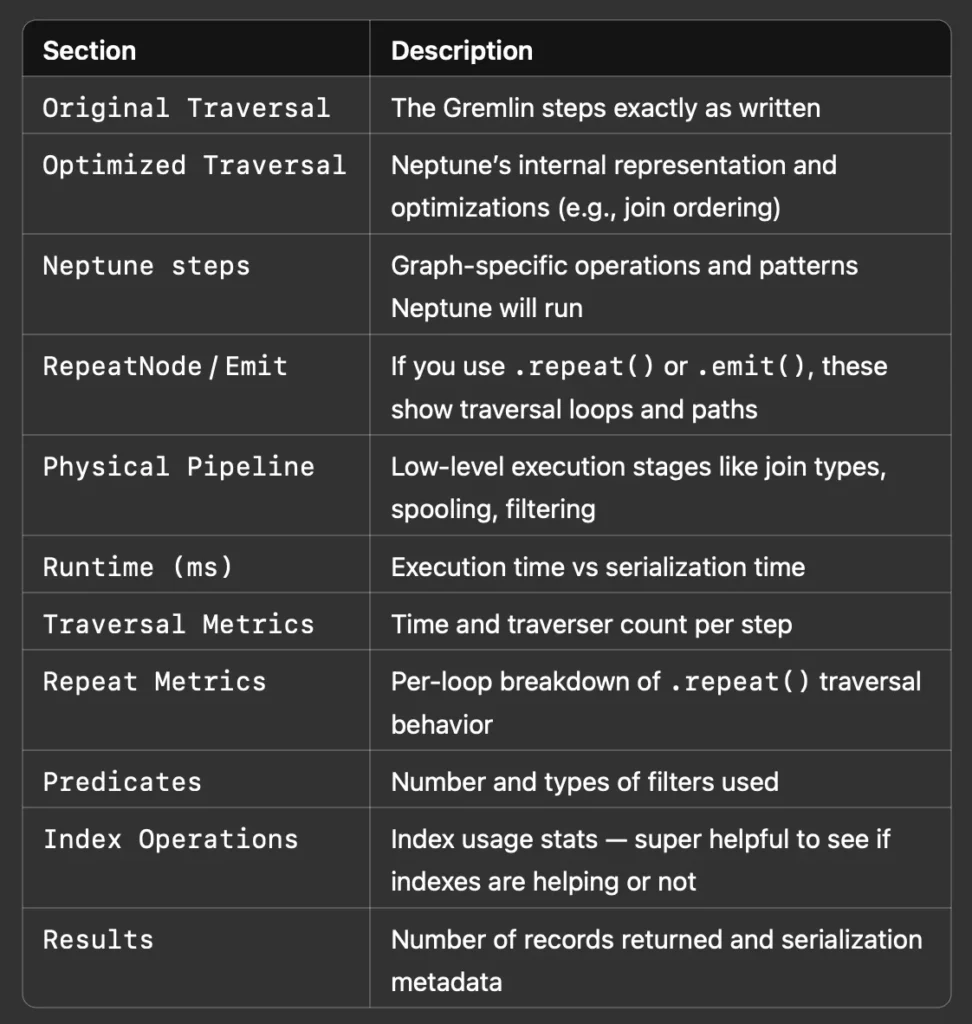
Let’s summarize each section so you can understand what it’s showing you:
SPARQL
In SPARQL, you use the explain=details parameter along with your query. Here’s how to get a detailed EXPLAIN plan using curl(you can also use the magic cell commands if running in Jupyter):
curl https://<your-neptune-endpoint>:<port>/sparql \

  -d "query=PREFIX ex: <https://example.com/> \

      SELECT ?person WHERE { ?person a ex:City ; ex:name \"London\" }" \

  -d "explain=details"
Sample Output
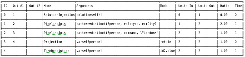
explain=details gives the most comprehensive view of how SPARQL queries are planned and executed internally in Neptune.
Let’s summarize each section so you can understand what it’s showing you:
openCypher
To generate an EXPLAIN plan in openCypher, use the explain=details parameter (you can also use the magic cell commands if running in Jupyter):
curl https://<your-neptune-endpoint>:<port>/openCypher \
  -d "query=MATCH (c:City {name: 'London'}) RETURN c" \
  -d "explain=details"
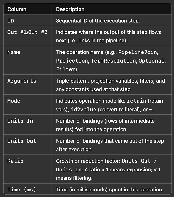
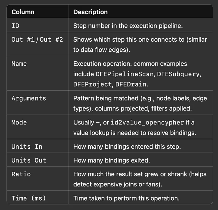
Sample Output
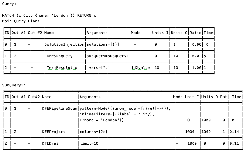
explain=details for openCypher shows execution stages, join logic, limits, and pattern estimates in tabular format, which is far more useful for performance analysis than the standard output.
Let’s summarize each section so you can understand what it’s showing you:
Interpreting the Output
The Neptune PROFILE output from Gremlin breaks down both execution stages and their costs. The Repeat Metrics are particularly useful for understanding traversal loops, which are common performance traps in graph queries. You can identify high-cost traversal segments and see how filter or path logic impacts execution.
For SPARQL and openCypher, the details mode turns static plans into detailed step-by-step analysis, with information like join types, projection order, filters, time cost per operator, and estimated vs actual data volumes.
Case Study: Gremlin Optimization in Action
Let’s break down a simple Gremlin example query. This query starts at the node that represents the city of London. From there, trace backward through all the incoming connections up to three steps away, ensuring you don’t revisit the same node twice. Then, go forward one step from wherever you land to find connected nodes. Pick only the events from those (i.e., have a type property set to “event”). Finally, return up to 50 matching results. This is the query written in Gremlin:
g.V()
  .has("name", "London")
  .hasLabel("city")
  .repeat(in().simplePath())
  .times(3)
  .out()
  .has("type", "event")
  .limit(50)
Explain Plan
>>> Neptune Profile Plan – Expand
*******************************************************
                Neptune Gremlin Profile
*******************************************************

Query String
==================
g.V().has("name", "London").hasLabel("city").repeat(in().simplePath()).times(3).out().has("type", "event").limit(50)

Original Traversal
==================
[GraphStep(vertex,[]), HasStep([name.eq(London)]), HasStep([~label.eq(city)]), RepeatStep(emit(false),[VertexStep(IN,vertex), PathFilterStep(simple), RepeatEndStep],until(loops(3))), VertexStep(OUT,vertex), HasStep([type.eq(event)]), RangeGlobalStep(0,50)]

Optimized Traversal
===================
Neptune steps:
[
  NeptuneGraphQueryStep(Vertex) {
    JoinGroupNode {
      PatternNode[(?1, <name>, "London", ?) . project ?1 .], {estimatedCardinality=2, indexTime=75, joinTime=4, hashJoin=true, actualTotalOutput=2} [1]
      PatternNode[(?1, <~label>, ?2=<city>, <~>) . project ask .], {estimatedCardinality=10000, indexTime=33, hashJoin=true, joinTime=0, actualTotalOutput=2} [1]
      RepeatNode {
        Repeat {
          PatternNode[(?3, ?5, ?1, ?6) . project ?1,?3 . IsEdgeIdFilter(?6) . SimplePathFilter(?1, ?3)) .], {estimatedCardinality=70000, hashJoin=true, indexTime=0, joinTime=5} [2]
        }
        Emit {
          Filter(false)
        }
        LoopsCondition {
          LoopsFilter([?1, ?3],eq(3))
        }
      }, annotations={repeatMode=BFS, emitFirst=false, untilFirst=false, leftVar=?1, rightVar=?3}
    }, finishers=[filter(type=event), limit(50)], annotations={path=[Vertex(?1):GraphStep, Repeat[Vertex(?3):VertexStep], Vertex(?4):VertexStep], joinStats=true, optimizationTime=519, maxVarId=9, executionTime=483} [3]
  },
  NeptuneTraverserConverterStep
]

Physical Pipeline
=================
NeptuneGraphQueryStep
  |-- StartOp
  |-- JoinGroupOp
      |-- SpoolerOp(100)
      |-- DynamicJoinOp(PatternNode[(?1, <name>, "London", ?) . project ?1 .], {estimatedCardinality=2, indexTime=75}) [1]
      |-- SpoolerOp(100)
      |-- DynamicJoinOp(PatternNode[(?1, <~label>, ?2=<city>, <~>) . project ask .], {estimatedCardinality=10000, indexTime=33}) [1]
      |-- RepeatOp
          |-- <upstream input> (Iteration 0) [visited=2, output=2 (until=0, emit=0), next=2]
          |-- BindingSetQueue (Iteration 1) [visited=250, output=250 (until=0, emit=0), next=250]
              |-- DynamicJoinOp(PatternNode[(?3, ?5, ?1, ?6) . ...]) [2]
          |-- BindingSetQueue (Iteration 2) [visited=950, output=950 (until=0, emit=0), next=950]
          |-- BindingSetQueue (Iteration 3) [visited=19500, output=19500 (until=19500, emit=0), next=0]
      |-- VertexStep(OUT)

      |-- FilterStep(type = event) [3]

      |-- LimitOp(50)

Runtime (ms)
============

Query Execution: 483.222
Serialization:   2798.304

Traversal Metrics
=================
Step                            Count  Traversers   Time (ms)
------------------------------------------------------------
NeptuneGraphQueryStep           50        50        403.187
NeptuneTraverserConverterStep   50        50         80.035

Repeat Metrics
==============
Iteration  Visited   Output    Until     Emit     Next
------------------------------------------------------
        0        2        2        0        0        2
        1      250      250        0        0      250
        2      950      950        0        0      950
        3    19500    19500    19500        0        0
------------------------------------------------------
             20702    20702    19500        0     1202

Warnings:
⚠ reverse traversal with no edge label(s) [2]
⚠ high fan-out detected in repeat [2]
⚠ filter applied late in traversal chain [3]
Neptune EXPLAIN Plan Shows
[x] shows where this information can be found in the above explain plan:
[1] Inefficient start: the first filter condition is against a parameter where the cardinality is low, whereas the second filter has a much higher cardinality. These filters could be reordered for better pruning. The higher the cardinality, the greater the range of possible values in the data set, which implies a smaller returned dataset due to fewer values matching. The aim is to have the smallest dataset returned first. For example, you have two filters on potentially 10,000 nodes each. One filter selects 50% of those nodes, and the other selects 10%. You want the 10% filter to be processed first so that only 1,000 nodes are passed to the next filter. If it’s processed the other way around, you pass five times as many nodes to the next filter condition, meaning more data is processed, leading to slower query times.
[2] .in() has no edge label which leads to scanning all incoming edges. The repeat traversal explodes in size (from 2 to nearly 20K nodes).
[3] The .out() and .has(“type”, “event”) filters are applied after this large expansion, which is inefficient.
Total traversal count: 20K+; lots of wasted effort.
Optimized Version
g.V()
  .hasLabel("city")
  .has("name", "London")
  .repeat(in("located_in").simplePath())
  .times(3)
  .out("hosts")
  .has("type", "event")
  .limit(50)
Improvements Made
- Added edge label filters to both .in() and .out()
- Moved .has(“type”, “event”) earlier to reduce downstream cost
- Preserved .simplePath() for cycle protection, but made it optional for testing
PROFILE Output After Optimization
>>> Neptune Profile Plan – Expand
*******************************************************
                Neptune Gremlin Profile
*******************************************************

Query String
==================
g.V().hasLabel("city").has("name", "London")
  .repeat(in("located_in").simplePath()).times(3)
  .out("hosts").has("type", "event").limit(50)

Original Traversal
==================
[GraphStep(vertex,[]),
 HasStep([~label.eq(city)]),
 HasStep([name.eq(London)]),
 RepeatStep(emit(false), [VertexStep(IN,[located_in]), PathFilterStep(simple), RepeatEndStep], until(loops(3))),
 VertexStep(OUT,[hosts]),
 HasStep([type.eq(event)]),
 RangeGlobalStep(0,50)]

Optimized Traversal
===================
Neptune steps:
[
  NeptuneGraphQueryStep(Vertex) {
    JoinGroupNode {
      PatternNode[(?1, <~label>, ?2=<city>, <~>) . project ask .], {estimatedCardinality=3000, indexTime=21, actualTotalOutput=7}
      PatternNode[(?1, <name>, "London", ?) . project ?1 .], {estimatedCardinality=1, indexTime=62, actualTotalOutput=1}
      RepeatNode {
        Repeat {
          PatternNode[(?3, <located_in>, ?1, ?) . project ?1,?3 . SimplePathFilter(?1,?3)] {estimatedCardinality=4500, hashJoin=true}
        }
        Emit { Filter(false) }
        LoopsCondition { LoopsFilter([?1, ?3], eq(3)) }
      }, annotations={repeatMode=BFS, emitFirst=false, untilFirst=false, leftVar=?1, rightVar=?3}
    },
    JoinGroupNode {
      PatternNode[(?3, <hosts>, ?4, ?) . project ?4 .], {estimatedCardinality=500, hashJoin=true}
      PatternNode[(?4, <type>, "event", ?) . project ?4 .], {estimatedCardinality=150, hashJoin=true}
    },
    finishers=[limit(50)],
    annotations={executionTime=192, optimizationTime=87, path=[Vertex(?1)->Repeat(?3)->Vertex(?4)]}
  },
  NeptuneTraverserConverterStep
]

Physical Pipeline
=================
NeptuneGraphQueryStep
  |-- StartOp
  |-- JoinGroupOp
      |-- DynamicJoinOp(PatternNode[(?1, <~label>, ?2=<city>, <~>) ...])
      |-- DynamicJoinOp(PatternNode[(?1, <name>, "London", ?) ...])
      |-- RepeatOp
          |-- Iteration 0: visited=1, output=1, next=1
          |-- Iteration 1: visited=35, output=35, next=35
          |-- Iteration 2: visited=85, output=85, next=85
          |-- Iteration 3: visited=120, output=120, next=0
      |-- DynamicJoinOp(PatternNode[(?3, <hosts>, ?4, ?) ...])
      |-- DynamicJoinOp(PatternNode[(?4, <type>, "event", ?) ...])
      |-- LimitOp(50)

Runtime (ms)
============
Query Execution: 172.329
Serialization:    817.502

Traversal Metrics
=================
Step                            Count  Traversers   Time (ms)   % Dur
---------------------------------------------------------------------
NeptuneGraphQueryStep            50        50         139.438   80.9
NeptuneTraverserConverterStep    50        50          32.891   19.1
                                TOTAL                  172.329

Repeat Metrics
==============
Iteration  Visited   Output    Until     Emit     Next
------------------------------------------------------
        0        1        1        0        0        1
        1       35       35        0        0       35
        2       85       85        0        0       85
        3      120      120        0        0        0
------------------------------------------------------
               241      241        0        0      121
Result:
Total traversed nodes: ~241 vs ~20,702
- Query time reduced by 60%+
- Reduced memory pressure and risk of timeout
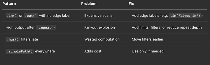
TL;DR — What to Look for in EXPLAIN/PROFILE
Tips & Tricks
- Push down filters: Apply filters as early as possible in your query.
- Use the right direction: Reverse your traversal if it leads to more selective starting points.
- Be cautious with OPTIONAL (SPARQL): These can dramatically increase plan complexity.
- Consider label cardinality: High-cardinality labels perform better as query roots.
- Don’t forget model design: Sometimes, performance issues are symptoms of poor graph structure.
Visualizing Query Plans
For large plans, consider writing a Python script that parses the JSON output and renders it as a tree using Graphviz or D3.js. It’s a great way to make the structure easier to digest and share with teammates.
Final Thoughts
Neptune’s EXPLAIN command is one of the most underused tools in the graph developer’s toolbox. Once you start using it, you’ll wonder how you ever worked without it. Understanding how the query planner thinks lets you shape your queries, and your graph itself, for better, faster results.
Now go forth and debug those query plans like a pro. 🕵️♀️
PS: If you’re interested in a follow-up deep dive on visualizing EXPLAIN plans or benchmarking query performance, let me know — I’m always up for some graph nerdery. Let me know here or in the comments.
![]()